Speculative decoding, from zero to DSpark

Big models generate slowly and verify fast. Speculative decoding exploits the gap. A post about how it works, and how DSpark pushes it into a real serving system.

Jul 10, 2026

Written with help from Muse Spark for drafting, editing, and figures. All the mistakes are its.

A new paper called DSpark came out recently (From the DeepSeek team,), and I wanted to understand what it adds beyond regular speculative decoding. The basic trick is to draft several tokens cheaply, then verify them with the big model in one pass. DSpark builds on that with two ideas: better long drafts, and a smarter way to decide how many drafted tokens to verify in production.

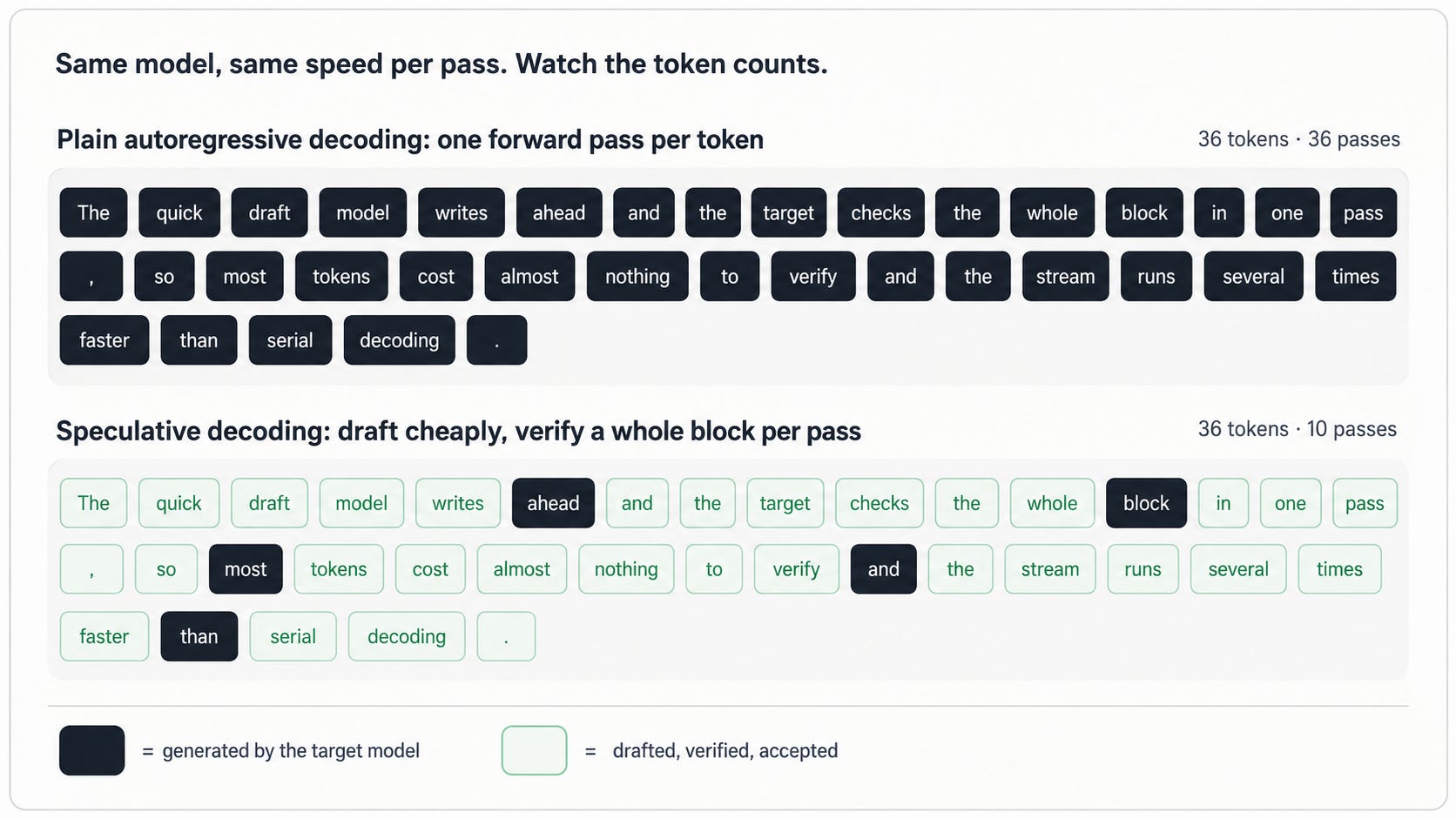
1. A full forward pass for every single token

An autoregressive language model produces text one token at a time. To generate token t+1 it needs a forward pass conditioned on everything up to token t.

To see whether that’s a problem, let’s follow one decoding step through the GPU and watch where the time goes. To generate one new token, the model has to produce its logits, the pre-softmax scores over the vocabulary. Getting them means every weight matrix in the model has to travel from the GPU’s main memory into the arithmetic units. That main memory is called HBM (High Bandwidth Memory), and it holds the model’s weights along with the KV cache, the stored attention state. For a 70B model in 16-bit, one token’s worth of logits costs about 140 GB of weight reads.

The arithmetic done with all that data is tiny by comparison: each weight participates in roughly one multiply-add per token. An H100 does on the order of a thousand trillion multiply-adds per second but reads only about 3 TB/s out of HBM. So the decoding step is memory-bound: its wall-clock time is set by how long the weight reads take, not by the math. The opposite regime, where the arithmetic itself is what you wait on, is called compute-bound. Decoding is nowhere near it, and that gap is the whole opportunity. In the memory-bound regime the arithmetic units are mostly idle: the multipliers finish their work instantly and then sit there while the next slab of weights streams in.

The loophole is that the weight reads are paid per forward pass, not per token. Push eight token positions through the same pass and the weights are read from HBM once, then multiplied against eight vectors instead of one. The memory traffic barely changes. You do eight times the arithmetic, but arithmetic was the idle resource anyway, so a pass over eight positions takes barely longer than a pass over one.

You already know this effect as the prefill/decode gap. Prefill is when the model ingests your prompt. All the prompt tokens are known up front, so they go through the model together, thousands of positions per pass, and the weight-read cost is split across all of them. Decoding generates one new token per pass and pays the full cost every single time.

Decoding can’t batch like prefill because the input at position t+1 is the token sampled at position t; it doesn’t exist until the previous pass finishes. But suppose someone handed you a guess for the next eight tokens. Now you do have all eight inputs, tentatively, and the big model can process them prefill-style in one pass. And the same pass gives the model its own next-token distribution at each of the eight positions. Those distributions are all it needs to go through the guess position by position and find where it stops being right. Verification is prefill-shaped. Generation is decode-shaped.

Who writes the guess? A smaller, cheaper model. That’s speculative decoding: everything in this post converts slow generation into fast verification plus a cheap guess.

2. Draft cheap, verify in parallel

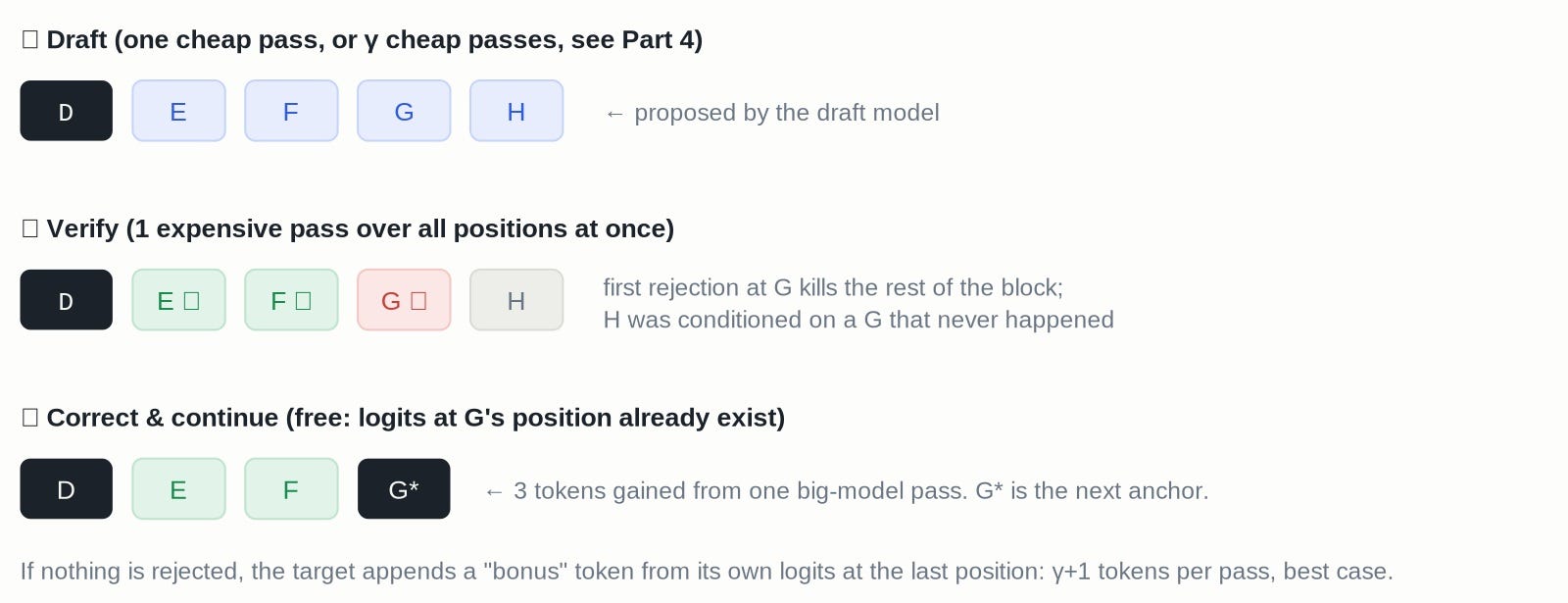
Speculative decoding runs as a loop: draft a few tokens, verify them, keep the good prefix, repeat. The version everyone uses is due to Leviathan et al. and Chen et al. A lightweight draft model proposes a block of γ candidate tokens. The target model runs one forward pass over the whole block and gets its own next-token distribution at every position. Then it walks the block left to right and decides, position by position, whether it agrees with the draft.

Say the last confirmed token is D. Call it the anchor: the confirmed token this round’s draft hangs off. The draft proposes E F G H. The target might accept E and F and reject G. A rejection isn’t wasted work: the target already computed a distribution at G’s position, so it samples a replacement G* from a corrected version of it. G* is called the correction token. Everything after the first rejection (H) is thrown away, because it was conditioned on a token that never happened.

If every draft token is accepted, the round earns one extra token for free: the pass also computed the target’s distribution at the position after the last draft token, so the target samples from it and appends the bonus token.

One speculative decoding round: draft several tokens, verify them in one target pass, keep the accepted prefix, then correct or continue.

The acceptance rule, and why the output is exact

The big claim of speculative decoding is that it’s lossless: the output tokens are distributed exactly as if the target model had generated them alone, temperature and all. This is a real guarantee, not an approximation, and it comes from a rejection-sampling rule. At position k, with draft distribution pᵈ and target distribution pᵗ, the drafted token xₖ is accepted with probability

\( P(\mathrm{accept}\ x_k)=\min\left(1,\frac{p^t(x_k)}{p^d(x_k)}\right)\)

In other words: when the target assigns the drafted token at least as much probability as the draft did, pᵗ(xₖ) ≥ pᵈ(xₖ), keep it always. When the draft over-sampled it, giving it more probability than the target does, keep it only in proportion pᵗ/pᵈ. On rejection, the replacement is sampled from the residual distribution norm(max(0, pᵗ − pᵈ)): max keeps the tokens where the target wanted more mass than the draft gave them, and norm rescales what’s left to sum to 1.

A nice consequence is that the per-position acceptance probability equals

\(P(\mathrm{accept})=1-\frac{1}{2}\lVert p^d-p^t\rVert_1\)

which says the drafter’s entire job is to stay distributionally close to the target. DSpark reuses this exact quantity later as a free training label. (Why the rule is exact, and why this distance is total variation rather than KL: Appendix A1 and A2.)

3. The latency equation

How much time does it take to produce one token? Speculative decoding pays per round, one draft plus one verification, and gets a variable number of tokens back, so its cost is time-per-round divided by tokens-per-round. Let τ be the average number of tokens you get per round (accepted draft tokens plus the bonus/correction token), T_draft the time to write the draft, and T_verify the time for the target’s verification pass. Then the latency per generated token is

\(L=\frac{T_{\mathrm{draft}}+T_{\mathrm{verify}}}{\tau}\)

That leaves three ways to go faster. You can draft faster, shrinking T_draft. You can draft better, raising τ by getting the drafter to agree with the target more often and for longer. Or you can verify smarter, and stop spending T_verify on draft tokens that were never going to survive. Most of the literature picks one of the three.

DSpark is unusual in going after two terms at once: τ with an architecture change (Parts 5 and 6), and T_verify with a scheduler (Parts 7 to 9). The second attack only makes sense once you stop thinking about a single user and start thinking about a serving system with hundreds of concurrent requests. But first, the standard menu of drafter designs.

4. Two ways to build a drafter

Autoregressive drafters (EAGLE, DeepSeek’s MTP (multi-token prediction)) are small language models that generate the draft one token at a time, each conditioned on the last. They produce coherent drafts, but the drafting cost scales linearly with the block size, T_draft ∝ γ. To keep the draft cheap they have to stay shallow (EAGLE-style drafters are often a single transformer layer) and keep γ small, which caps both the block length and how much the drafter can know.

Parallel drafters (Medusa, and more recently DFlash) fill in all γ positions in a single forward pass. Feed in the anchor token plus a row of mask tokens, read out logits everywhere at once, diffusion-style. Now T_draft is nearly independent of γ, so you can afford a much deeper drafter (DFlash uses 5 layers where EAGLE uses 1) and much longer blocks (γ = 16 costs about what γ = 4 costs).

DFlash, the parallel drafter DSpark builds on, is worth describing in some detail because DSpark reuses its entire skeleton. The drafter is a small transformer, 5 layers in the paper. Its input for one drafting round is the embedding of the anchor token (the last token the target actually confirmed) followed by mask-token embeddings, placeholders for the positions to be filled in. All positions attend to each other bidirectionally, and one forward pass produces logits for every position in the block. The drafter doesn’t even own an embedding table or an output head. It borrows the target model’s, frozen.

Its central trick is how it sees the conversation, called KV injection. While the target processes the context, hidden states from a few of its layers are saved, projected down into the drafter’s width, and prepended to the keys and values of every drafter layer, so each draft position attends to the target’s own internal representation of everything said so far. All of it is computed once, at prefill, and reused every round. The drafter isn’t understanding the conversation with 5 layers of its own; it’s reading the big model’s notes, which is a big part of why it can imitate a model thousands of times larger. (Mechanics and a diagram: Appendix A3.)

So a parallel drafter is both faster to run and free to be deeper. That sounds like it should win outright, but it doesn’t…

Larger draft blocks help only when acceptance stays high; otherwise most late draft tokens are wasted....

5. Where parallel drafters break: the multi-modal collision

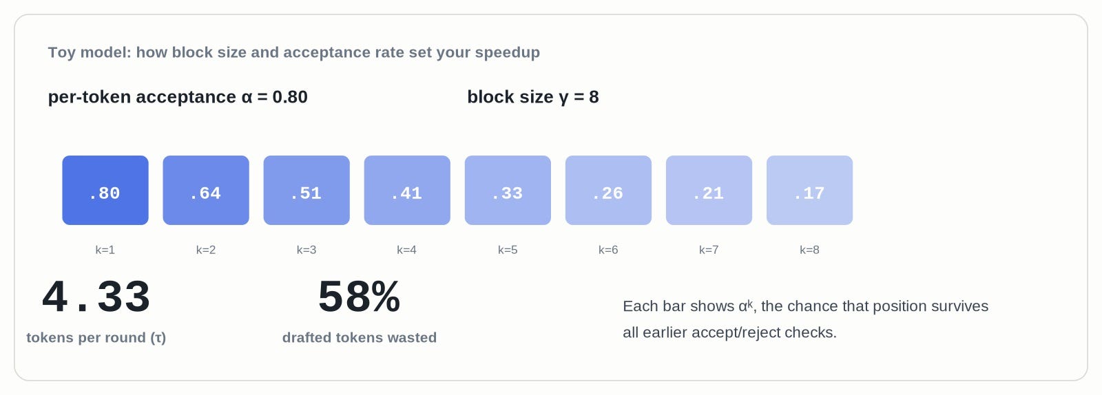
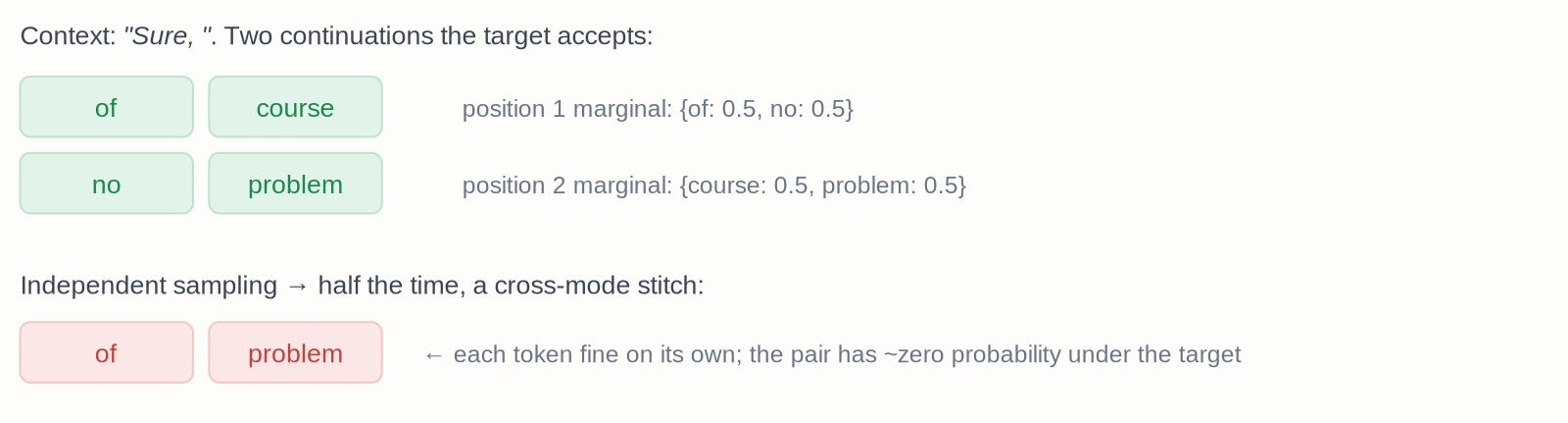
A parallel drafter predicts every position independently, in one shot. Position 3 can’t see what position 2 actually sampled, only the shared context. So when the context admits several equally good continuations, each position hedges across all of them.

Take the context “Sure, “. The target model is happy with either of course or no problem. A parallel drafter, sampling each position from its marginal, can happily emit of problem or no course: fragments of two valid answers stitched into an invalid one. This is the multi-modal collision problem, known since the non-autoregressive machine translation days (Gu et al., 2018). Each token is individually plausible, the combination is garbage, and the target rejects it.

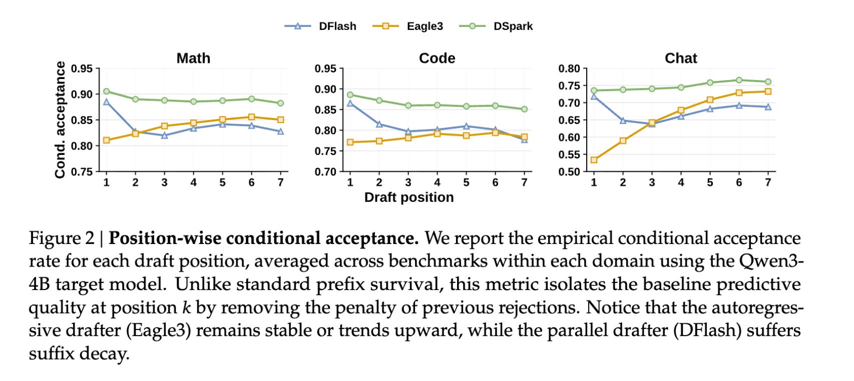
A parallel drafter can mix pieces of different valid continuations, producing a sequence the target rejects....

The damage shows up as suffix decay: acceptance falls off rapidly with position in the block. The paper measures this with a nice metric, position-wise conditional acceptance: at position k, only count cases where positions 1…k−1 were all accepted, then ask how often k is accepted too. This strips out the compounding survival penalty and shows the drafter’s raw predictive quality at each depth.

Here are the curves (Qwen3-4B target, chat domain):

Why DFlash still gets the longer accepted length

The curves make Eagle3 look like the better drafter everywhere past position three. And yet, on accepted length, DFlash beats it on nearly every benchmark in the paper. The mismatch is explained by how verification scores a block.

Verification accepts a prefix and discards everything after the first rejection, so the expected haul per round compounds multiplicatively. Write the expected accepted count in terms of the conditional acceptance rates c₁, c₂, …:

\(\mathbb{E}[\mathrm{accepted}]\approx c_1+c_1c_2+c_1c_2c_3+\cdots\)

Every term contains c₁, so raising c₁ by 10% grows the entire sum by 10%, while raising c₆ only moves the last couple of terms. A rejection at position 1 erases the whole block; a rejection at position 6 erases one or two tokens. Whatever a drafter is good at, being good at position 1 is worth several times more than being good anywhere else.

And position 1 is where the deep parallel drafter has its edge. No draft tokens exist yet at the first position, so both drafter types condition on the same thing, the verified context, and dependency modeling buys nothing there. What decides position 1 is raw capacity, and the latency budgets are lopsided: the autoregressive drafter runs once per position and must stay shallow (Eagle3 is one layer), while the parallel drafter runs once per block and affords five layers plus KV injection.

6. DSpark idea #1: bolt a bigram onto the parallel drafter

The obvious fix for suffix decay is to make the drafter autoregressive again, but then you’re back to T_draft ∝ γ. DSpark adds autoregression only where it costs almost nothing. The expensive part, the 5-layer KV-injected DFlash backbone, runs fully parallel as before: one pass, producing hidden states h₁…hᵧ and base logits U₁…Uᵧ for every position. After that, a small sequential head passes over the block left to right and adds a correction to each position’s logits, and the correction depends on the tokens already sampled before it:

\(p_k(v\mid x_0,x_{<k})=\operatorname{softmax}\left(U_k(v)+B_k(x_0,x_{<k},v)\right)\)

In this formula, Uₖ is what the parallel backbone already gave us: the base logits for position k, one score per candidate token v over the vocabulary (V ≈ 10⁵ tokens), so Uₖ(v) is token v’s score. Bₖ(x₀, x<k, v) is the sequential head’s correction to that score, and it’s the only term allowed to look at the block’s history: the anchor x₀ and the draft tokens x<k already sampled at earlier positions.

The default B is a small Markov head. It throws away everything except the immediately preceding token: the correction becomes B(xₖ−₁, ·) ∈ ℝV, a full vector of logit corrections, one per candidate next token, selected by which token came just before. Written out as a table that’s a V×V matrix, a row per possible previous token and a column per possible next token. In other words, a learned bigram model, stored factorized at rank 256: per position the sequential loop costs one table lookup plus one small matrix-vector product, invisible next to the target’s verification pass. And it is learned with the rest of the drafter rather than counted from a corpus (dimensions and training: Appendix A4).

Back to the collision. The backbone, in parallel, gives position 1 as {of, no} and position 2 as {course, problem}. The sequential loop samples position 1 first and gets of. When it moves to position 2, the bigram bias for “of” boosts course and suppresses problem, so the drafter no longer stitches “of problem” together.

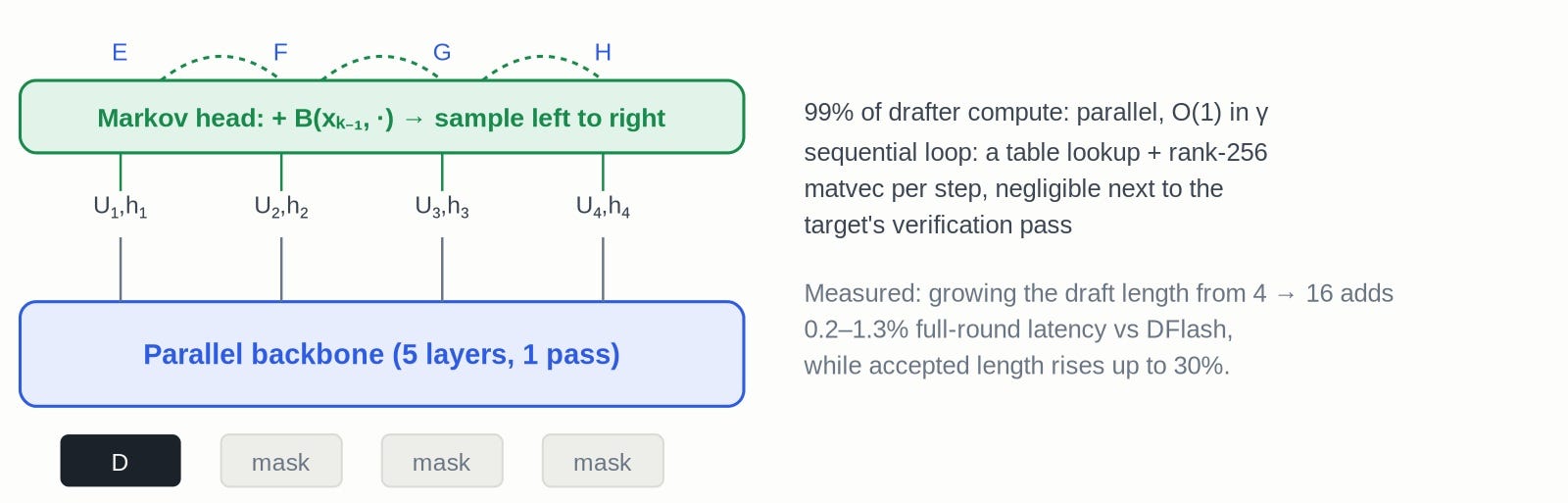
DSpark keeps the expensive drafter computation parallel, then adds a cheap sequential Markov head to improve within-block coherence.

Does one token of memory suffice? The authors also try an RNN head, a small gated recurrence that carries the whole within-block prefix instead of just the last token. It helps only marginally, and only at long blocks. I think that near-null result is the most useful thing in the paper: suffix decay in parallel drafters is mostly a problem of adjacent-token incoherence, not of missing long-range information.

Through KV injection (Part 4), every draft position already sees the target’s representation of the whole conversation. The missing piece is what the neighboring positions sampled, and that doesn’t exist until after the forward pass is over. Only something that runs at sampling time can close that gap, and a bigram is the smallest such thing.

Across Qwen3-4B/8B/14B, DSpark’s macro-average accepted length comes out 27–31% above Eagle3 and 16–18% above DFlash, and a 2-layer DSpark already beats the 5-layer DFlash, so the gain comes from the dependency modeling and not from extra parameters. On the conditional-acceptance curves, DSpark opens where DFlash opens and stays flat where Eagle3 stays flat.

7. The serving problem: draft tokens compete for batch space

Everything so far was a single-user story: one request, one GPU, minimize that one user’s latency. In production the target model is shared. One copy serves hundreds of users at once, and each of its forward passes processes a batch. The batching is done by the serving engine, the software layer that owns the GPU and runs the model; vLLM and SGLang are the open-source examples, and DeepSeek runs its own. Each pass, the engine collects the pending tokens of many requests and pushes them through together: the amortize-the-weight-reads trick from Part 1, applied across users instead of across positions.

But the batch is a shared, finite resource. A small batch keeps the pass memory-bound, so extra tokens ride along at no cost (Part 1). Keep adding tokens though, and at some batch size the arithmetic units stop being the idle party; past that point, every additional token makes the pass measurably slower for everyone in it. This gives every engine a characteristic curve, SPS(B): steps per second as a function of how many tokens the batch holds. It stays flat while the pass is memory-bound and falls once the batch pushes it into compute-bound territory, the two regimes from Part 1.

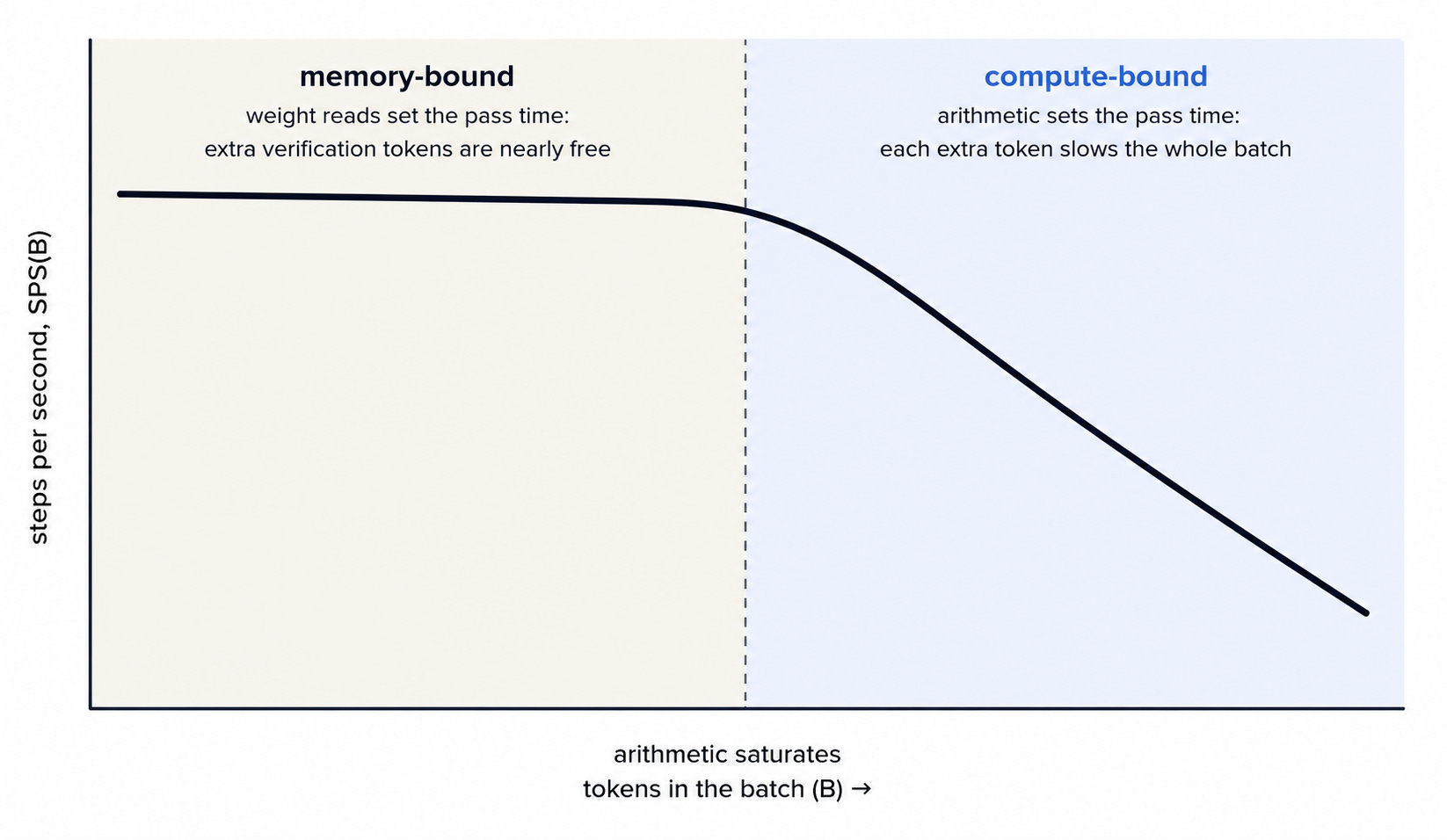
Extra verification tokens are nearly free while the batch is memory-bound, but costly once the system becomes compute-bound.

Every draft token a request submits for verification takes up one token-slot in the batch, and a rejected token wastes its slot. On the flat part of the curve that waste is harmless, so even a 20% long shot is worth checking. On the steep part, the same token contributes 0.2 expected tokens while slowing down the several hundred others sharing the pass, and it isn’t worth the slot.

The right amount of verification also depends on the content. Drafters do well on structured text and badly on open-ended text: on Qwen3-4B the paper measures roughly 5.6 accepted tokens per round on math, 5.1 on code, 3.5 on chat. A single fixed length is therefore wrong in both directions at once, wasting slots on chat requests whose late tokens were never going to be reached and cutting short code requests that could have gone longer.

Before this paper, the DeepSeek’s production system drafted a single token per round, the MTP-1 setup, even though they had already built multi-token drafters (MTP-3, MTP-5). With a static 3-token draft, every request adds 3 tokens to every batch whether the load or the content justifies it, and at production concurrency many of those tokens are late-position chat tokens headed for rejection. The batches grow, every pass slows, and the slowdown across all users outweighs the extra accepted tokens: total throughput drops. Production stayed at the largest setting that never backfired, one token per round, at a price: at γ = 1 a round yields at most two tokens, the draft plus the bonus, so the ceiling is roughly a 2x speedup and everything Part 4 built for long parallel blocks goes unused.

The way out of that dilemma is to stop picking one length for everyone and instead decide per request, per step: given the load right now, how many of this request’s drafted tokens deserve a batch slot? The drafter has already produced its full γ-token block, so that cost is sunk; the only choice is which of those tokens get slots, and whatever is cut is dropped unseen. Deciding needs a per-token estimate of the chance a slot pays off, plus a rule turning those estimates and the SPS curve into lengths.

8. DSpark idea #2: choose verification lengths by expected throughput

The scheduler is the part of the engine (Part 7) that decides, before each forward pass of the target model, what goes into that pass: which requests participate, and (the new degree of freedom here) how many draft tokens each request contributes. It answers Part 7’s question once per step, for the whole batch at once.

For one verification step, there are R active requests, each with a freshly drafted γ-token block, and the scheduler has to pick a verification length ℓᵣ ∈ {0, …, γ} for every request r: verify the first ℓᵣ draft tokens and drop the rest. A choice of lengths is judged by the expected token throughput of the whole system for this step:

\(\max\ \Theta=\tau\cdot \mathrm{SPS}(B),\quad \tau=\sum_r\left(1+\sum_{j\le \ell_r}a_{r,j}\right),\quad B=\sum_r(1+\ell_r)\)

SPS(B) is the Part 7 cost curve; the engine measures it once at startup by timing passes at a range of batch sizes and keeps the results as a lookup table. τ is the expected number of output tokens the pass will produce for the whole batch, i.e. Part 3’s per-request τ summed across all R requests. The two +1s are both the anchor: even at ℓᵣ = 0 a request still sends one token through the pass and gets one token back, the bonus or correction from Part 2. Each admitted draft token at position j then adds aᵣ,ⱼ to τ: the probability that it survives verification and actually ends up in the output. Expected tokens per step times steps per second gives expected tokens per second. The one missing part is those survival probabilities (a_r,j)

The confidence head

What does it mean for a slot to pay off? A draft token survives verification if the left-to-right check actually reaches it (every earlier token in the block was accepted) and accepts it too. “Reaches it” is the price of batched verification: the whole block is checked in one pass, but acceptance is prefix-only, so a rejection at position 3 means positions 4 and onward are discarded without ever being checked, however good their tokens were.

To do that, they use a confidence head, which outputs one scalar per position, cₖ, the conditional piece of survival: the probability that position k is accepted given that the check reached it. This is the same conditional acceptance rate the Part 5 curves measured, now predicted per token instead of averaged over a benchmark. The head itself is small. It reads the backbone hidden state plus the Markov embedding of the previous token and runs them through a single linear projection and a sigmoid. Its training label is free: the exact acceptance probability from Part 2 is computable at every training step and used directly as a soft label (Appendix A4).

Because the cₖ are conditionals, the chain rule turns them into full survival probabilities for free:

\(a_k=P(\mathrm{prefix}\ 1{:}k\ \mathrm{all\ accepted})=\prod_{i\le k}c_i \)

These aₖ, computed per request, are exactly the aᵣ,ⱼ the objective consumes, with one requirement: the arithmetic only works if the scores are calibrated, meaning a token scored 0.8 really is accepted about 80% of the time. Raw heads are overconfident; per-position temperature scaling shrinks the predicted-versus-observed gap from 3–8% to about 1% (Appendix A5).

Picking all R lengths at once sounds combinatorial, but the survival probabilities have a property that makes it easy. Within a request, aᵣ,ⱼ = cᵣ,₁·cᵣ,₂⋯cᵣ,ⱼ is a product of numbers between 0 and 1, so tacking on another factor can only shrink it: aᵣ,₁ ≥ aᵣ,₂ ≥ … ≥ aᵣ,ᵧ. In other words, surviving to j+1 requires surviving to j first, so it’s the stricter condition.

That ordering is what licenses a greedy algorithm. Extending request r’s length from j−1 to j adds exactly aᵣ,ⱼ to τ and exactly one token to B, a gain and a cost both known in advance. So pour all candidate extensions from all requests into one pool, sort by aᵣ,ⱼ, and admit from the top, recomputing Θ after each admission (a table lookup). The within-request constraint (you can’t verify position 3 without positions 1 and 2) enforces itself: since each request’s survival probabilities are already in decreasing order, its position-2 candidate always sits above its position-3 candidate in the global sort.

When the batch is nearly empty, SPS(B) sits on its flat stretch, admitting another token raises τ almost for free, and the scheduler verifies long: 4–6 tokens per request in the paper’s numbers. As the batch fills, each admitted token drags SPS down, only tokens whose survival probability beats the drag get in, and the budgets shrink. Within one batch, a code request at 0.9 confidence keeps a long verification while a chat request whose confidence collapses by position 2 gets cut there, with no threshold set anywhere.

A version of this that breaks losslessness

Losslessness needs one more condition beyond the accept/reject rule of Part 2, and this one falls on the scheduler: whether token k gets admitted for verification must not depend on the value of token k. The proofs call this non-anticipation. Fixed verification length satisfies it trivially, but a length chosen by the greedy search above can violate it.

The violation runs through the confidence head, which reads the Markov embedding of the previous sampled token: c₂, and therefore a₂, is a function of which x₁ was drawn. The block is fully sampled before scheduling (Part 7), so a₂ is available; the question is whether the scheduler may consult it. Suppose it evaluates the whole admission path and takes the argmax: Θ at lengths 0, 1, 2. The length-2 value used a₂, which used x₁. So the comparison that decides whether x₁ is admitted at all already depends on which x₁ was drawn, and draft tokens that lead to confident continuations get admitted more often than ones that don’t.

For example, with a two-token vocabulary: the target wants {A: 0.7, B: 0.3}, the drafter samples from {A: 0.5, B: 0.5}, and suppose drawing A leads to a high c₂ while drawing B leads to a low one, so the argmax scheduler admits the draft after drawing A and skips it after drawing B. When A is drawn (probability 0.5), it is admitted and accepted with probability min(1, 0.7/0.5) = 1. When B is drawn, nothing is admitted and the target samples fresh from {0.7, 0.3}. Total: P(output = A) = 0.5 + 0.5 × 0.7 = 0.85 instead of 0.7.

The clean algorithm’s solution is an early-stopping break: walk the sorted admission path and stop at the first admission that lowers Θ. Then the decision about position k is finalized before anything computed from xₖ is ever consulted, and the proof goes through.

9. Making it run in a real engine

Inside DeepSeek’s actual engine, the Part 8 algorithm breaks in two places. The first is that the SPS curve isn’t smooth. Kernels are tuned for particular batch shapes, so pass time jumps at tile-size and dispatch boundaries rather than rising gradually. On a jagged curve the early-stopping break turns into a liability: Θ can dip at a cliff and recover just past it, and a search that quits at the first dip strands the system at a local optimum.

The second is about timing. A modern engine assembles the next pass while the current one runs, and with CUDA-graph replay the next batch size has to be fixed before the current pass finishes. The Part 8 scheduler can’t meet that deadline, since it needs the current step’s confidence scores, and those don’t exist until the step is done. Run it synchronously and the GPU stalls between every pair of steps.

The deployed version works around both problems by computing the batch’s capacity a couple of steps ahead of time. The scheduler fixes K, the number of tokens the next pass can afford to verify, using confidence scores from two steps back, so it’s ready before the pass launches. The tokens that actually fill those K slots are still chosen at the last moment from the current step’s real confidence scores, by sorting the live candidates as in Part 8 and keeping the top K.

This design also settles the losslessness question from Part 8, where the danger was that computing the cut-off consulted downstream token values. Here the cut-off is K, fixed from two-step-old data before any of this step’s tokens existed, and the fresh ranking that fills the slots consults only tokens earlier in the block, never token k itself or anything after it. That is exactly what non-anticipation demands, so it holds by construction, the early-stopping break can go, and the search over the jagged curve can run globally to the true maximum. The same design choice that fixed the pipeline stall also restored exactness; my guess is the pipeline constraint came first and the losslessness argument was noticed after the fact.

The live-traffic numbers

Deployed on DeepSeek-V4-Flash and V4-Pro under real user traffic, against the incumbent MTP-1:

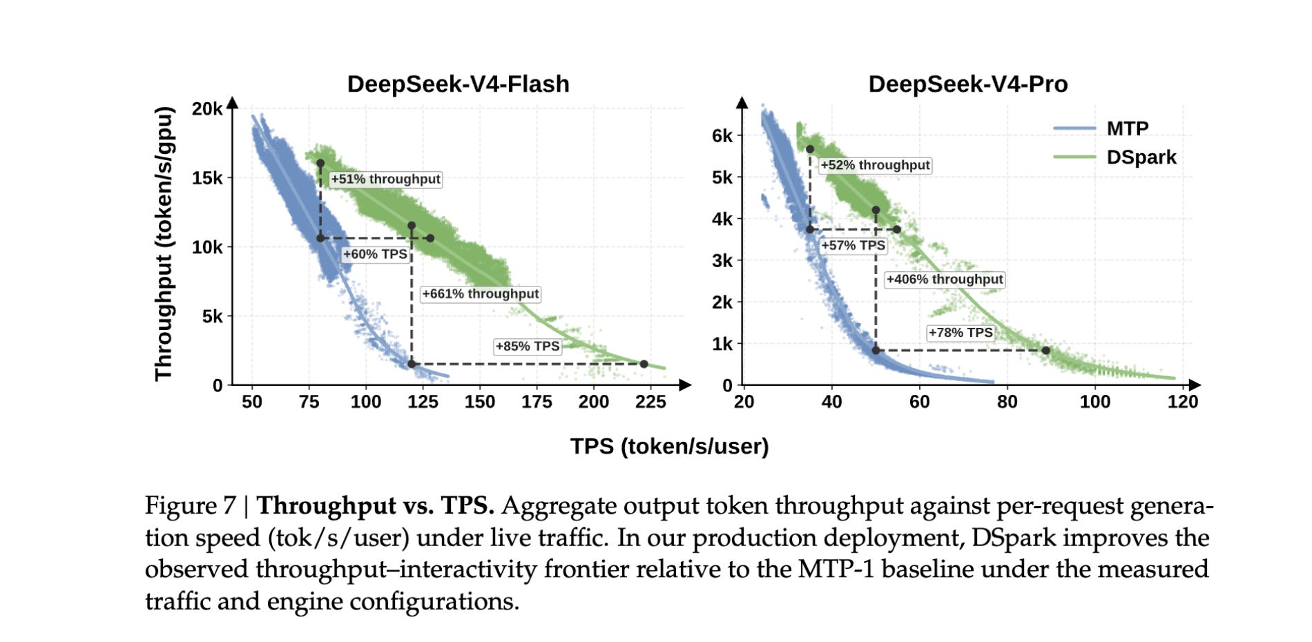
The paper’s Figure 8 shows that at moderate concurrency the average verification budget sits at 4–6 tokens per request, and as concurrency rises the scheduler shrinks it, dropping low-confidence tokens before they occupy batch slots.

Next Steps

A few things the paper leaves open. The SPS table is profiled once and indexed by batch size alone, but real per-step cost also depends on the batch’s context-length mix, so a 1-D curve is an approximation. The confidence head is trained on the analytical acceptance labels under teacher-forced prefixes but deployed on sampled ones. That’s a train/inference mismatch. Calibration is fit on a held-out set, and live traffic drifts; whether the head stays calibrated online isn’t reported. And the drafter still burns a full γ-block forward on every request, even hopeless ones. The scheduler prunes verification, not drafting.

10. What to actually remember

The important thing about DSpark is not just that it makes speculative decoding faster. Earlier work mostly asked how to build a better drafter: make it cheaper, deeper, or more accurate. DSpark shows that this is only half the story. In a real serving system, the question is not “how many tokens can I draft?” but “which drafted tokens are worth spending target-model batch capacity on right now?” The paper’s two main ideas answer both sides of that question: a semi-autoregressive Markov head makes long parallel drafts much more coherent, and a throughput-aware scheduler decides how much of each draft to verify under the current load.

A. Appendix: the fine print

Details that back the main text but aren’t needed to follow it.

A1. Why the rejection rule is exact

Check any token v. It reaches the output two ways: drafted and kept, or rejected and resampled. If pᵗ(v) ≤ pᵈ(v), the kept route alone contributes pᵈ(v) · pᵗ(v)/pᵈ(v) = pᵗ(v) and the residual has zero mass on v. If pᵗ(v) > pᵈ(v), the kept route contributes pᵈ(v) and the resample supplies exactly the missing pᵗ(v) − pᵈ(v), because the overall rejection probability equals the residual’s normalizer. Either way: pᵗ(v). The same accounting shows why the replacement can’t simply be drawn from pᵗ: acceptance already gave every token min(pᵗ, pᵈ), so the rejection branch may supply only the shortfall. With pᵗ = {A: 0.7, B: 0.3} and pᵈ = {A: 0.5, B: 0.5}, resampling from the full pᵗ would give P(A) = 0.5 + 0.2 × 0.7 = 0.64 instead of 0.7, tilting the output toward the tokens the draft over-proposed.

A2. The distance is total variation, not KL

The distance in the acceptance formula is total variation, not KL. TV is symmetric, so there is no forward or reverse version of the statement, and Pinsker’s inequality (TV ≤ √(KL/2)) says pushing either KL down also pushes acceptance up. The paper’s distillation loss skips the surrogate entirely and minimizes the L1 term directly, so it is optimizing the acceptance rate itself.

A3. KV injection, in detail

Its central trick is how it sees the conversation, called KV injection. The drafter never reads the context as text, and it never runs its own forward pass over it. Instead it recycles work the target already did. When the target processes the context, every one of its layers produces a hidden state for every token: a vector encoding that token after the layer has mixed in information from everything before it. DFlash saves these hidden states from a handful of target layers; different depths carry different levels of abstraction, from surface features early to semantics late, so the drafter gets a cross-section rather than a single view. For each context token, the saved vectors are concatenated across the chosen layers and passed through a learned projection down into the drafter’s much smaller hidden size, giving one compact context vector per context token. All of this is computed once, during the target’s prefill, and reused on every drafting round after that.

These vectors enter the drafter through attention. Recall the split of roles there: queries ask, keys and values are what gets read. In every layer of the drafter, the context vectors are projected into keys and values and prepended to that layer’s own keys and values, so from a draft position’s point of view they behave like extra tokens it can attend to. The draft positions do the querying; the target’s representations do the answering. Each draft position therefore sees two things at once: the other positions in its block, and the target’s own internal summary of everything said so far, at several depths. The drafter isn’t trying to understand the conversation with 5 layers of its own. It’s reading the big model’s notes, and the notes were written by the very network it’s trying to imitate, which is a big part of why a 5-layer model can predict what a model thousands of times larger will say next.

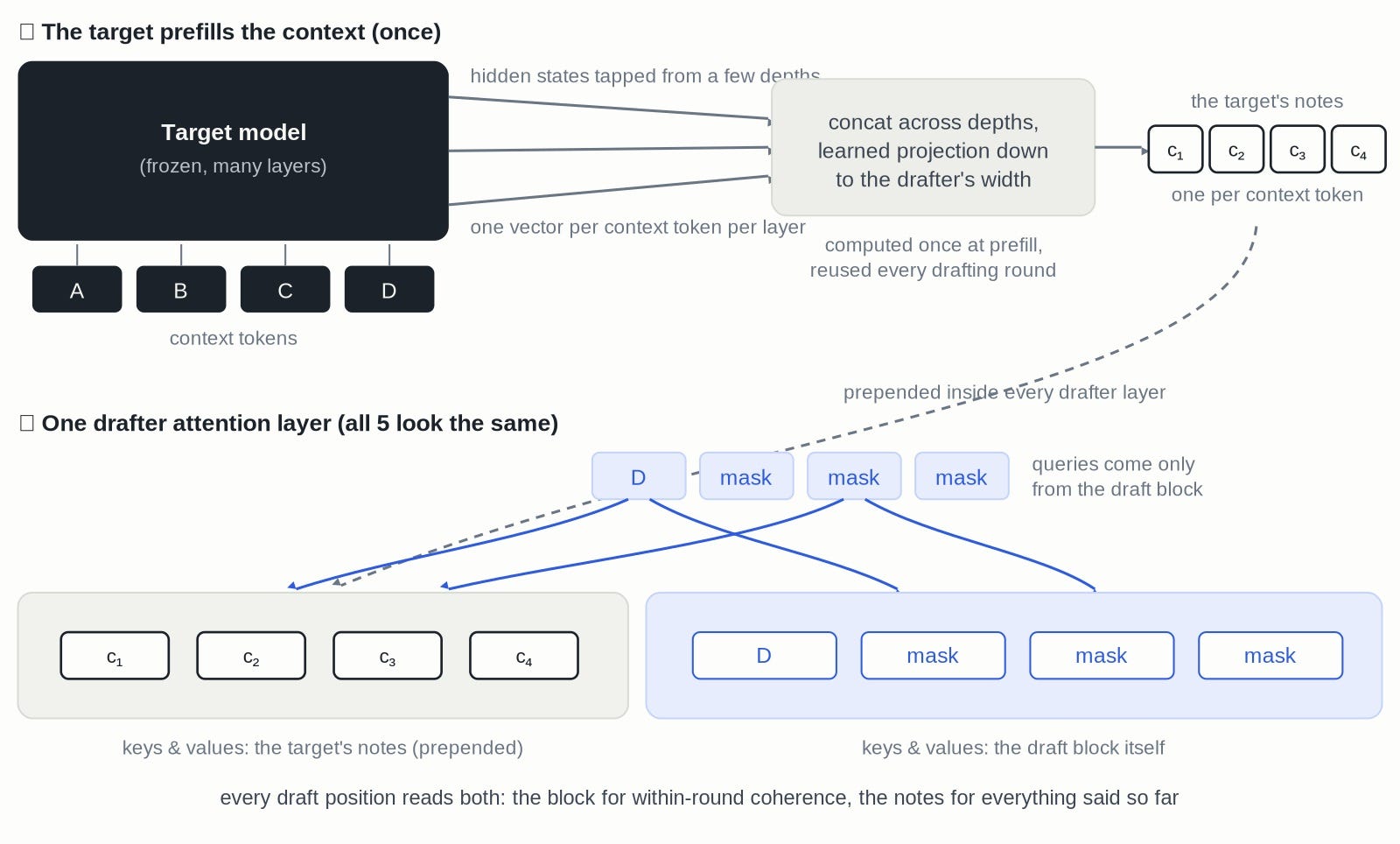
One construction detail: in the original DFlash the anchor plus γ masks go in and only the mask positions are predicted; DSpark trims this to anchor plus γ−1 masks and predicts at the anchor slot too, which saves a little compute at the same quality.

A4. The Markov head and the confidence head: dimensions and training

At this vocabulary size the bigram table would have ~10¹⁰ entries, so it’s stored factorized: B = W₁W₂, with W₁ ∈ ℝ^{V×256} and W₂ ∈ ℝ^{256×V}. Row xₖ−₁ of W₁ is a 256-dimensional embedding of the previous token (the paper’s Markov embedding, which the confidence head in Part 8 also reads), and multiplying it by W₂ expands it back to a V-dimensional correction. Per position: one table lookup plus one 256-by-V matrix-vector product.

W₁ and W₂ are not counted from corpus statistics. They are learned by gradient descent along with the rest of the drafter, trained to imitate the frozen target’s outputs, with Part 2’s TV distance as part of the loss.

The confidence head’s training label is free. Part 2 showed that the acceptance probability at a position is exactly 1 − ½‖pᵈ − pᵗ‖₁. Training the drafter already computes both distributions: the frozen target runs on the training data to provide supervision, which yields pᵗ at every position, and pᵈ is the drafter’s own output. So the true acceptance probability is available in closed form at every training step, and the confidence head is supervised directly with it as a soft label, without ever simulating an accept/reject decision.

A5. Calibrating the confidence head

A confidence head is calibrated if its numbers mean what they say: of all the tokens it scores 0.8, about 80% should actually be accepted. Simpler schemes don’t need this. A threshold rule like “drop everything below 0.4” only compares scores to a cutoff, so it works as long as better tokens get higher scores, even if every score is inflated. DSpark’s scheduler does arithmetic with the scores. It multiplies them into survival probabilities and sums those into an expected token count for the whole batch, so if the head says 0.9 where the truth is 0.7, the count is wrong and the scheduler ends up maximizing a throughput that doesn’t exist. Neural confidence estimates are, reliably, overconfident in exactly this way.

The fix is temperature scaling with one twist, which the paper calls Sequential Temperature Scaling. Because the scheduler consumes cumulative products, aₖ = c₁⋯cₖ, the calibration targets the products rather than the raw scores: walking left to right, each position gets one temperature, fit on held-out data to shrink the gap between the predicted and the observed acceptance of the cumulative product, with earlier positions held fixed. Temperature scaling only rescales scores, it never reorders them, so the ranking the head learned survives. The average gap between predicted and observed acceptance drops from 3–8% to about 1%.

A6. The empty-system limit

In the limit of an empty system, the maximization says to verify the entire γ-token block, since an admitted token can only add to τ. Light-load speed is therefore capped by γ and by drafter quality rather than by the scheduler, which is part of why Part 6’s fight to keep acceptance high at long blocks matters. The one cost light load doesn’t forgive is T_{draft}, paid every round regardless of what gets verified.

Source: Cheng et al., DSpark: Confidence-Scheduled Speculative Decoding with Semi-Autoregressive Generation (DeepSeek-AI & Peking University, 2026). Figures in this post are stylized redraws of the paper’s Figures 1, 2, and 7; all numbers are from the paper. DeepSeek released the DSpark checkpoints for the V4 preview models along with DeepSpec, a training repo where Eagle3, DFlash, and DSpark are all trained on the same data, so the baselines in this comparison are held fixed for once. Background reading: Leviathan et al. and Chen et al. (2023) on speculative sampling; Gu et al. (2018) on non-autoregressive generation and multi-modal collision; Li et al. on the EAGLE series; Chen et al. (2026) on DFlash.

The Information Bottleneck

Discussion about this post

Ready for more?