
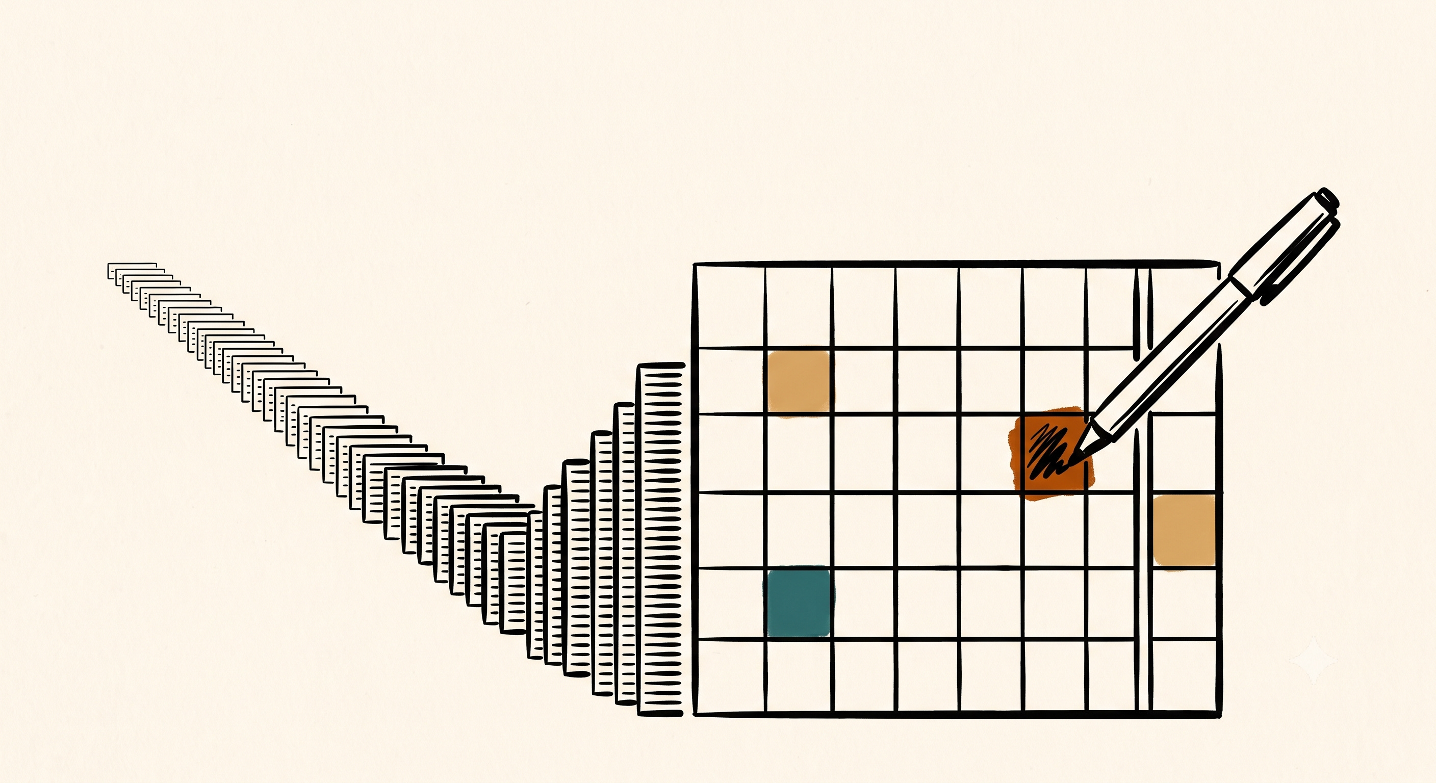
Editing a Compressed Memory
Linear attention compresses memory into one fixed-size matrix. The hard part is editing it without scrambling everything else.

Written with help from Claude for drafting, editing, and figures. All the mistakes are its.
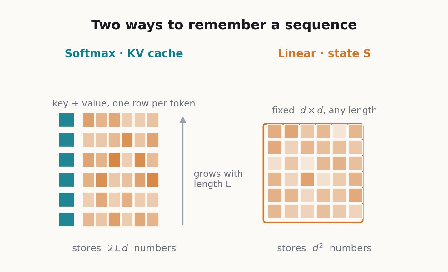
A Transformer remembers by keeping everything. Every token it has read stays in the KV cache, and any later token can look back at any earlier one exactly. That is why attention is so good at recall, and why its memory and compute grow with the length of the context.
Linear attention makes the opposite bet. It throws the cache away and keeps a single fixed-size matrix: a running summary that every new token updates and every query reads. Memory stops growing and decoding gets cheap. But a fixed-size summary cannot hold an unbounded number of facts cleanly, so writing something new can disturb what is already stored. Almost all the recent progress here (DeltaNet, Gated DeltaNet, KDA, and now Gated DeltaNet-2) is about making that write more surgical.
This post builds the whole thing from the ground up. You do not need to know any of these models going in; just linear algebra and a rough sense of what attention does. Shape of the argument
A fixed-size state is an associative memory built by summing key–value outer products, and reading it is content-addressed lookup.
Because it is fixed-size, overlapping keys interfere. That is the one limitation everything else fights.
Giving an old key a new value is the hard case. Adding leaves the stale value behind; replacing the matrix destroys every other fact; the delta rule does the surgical thing.
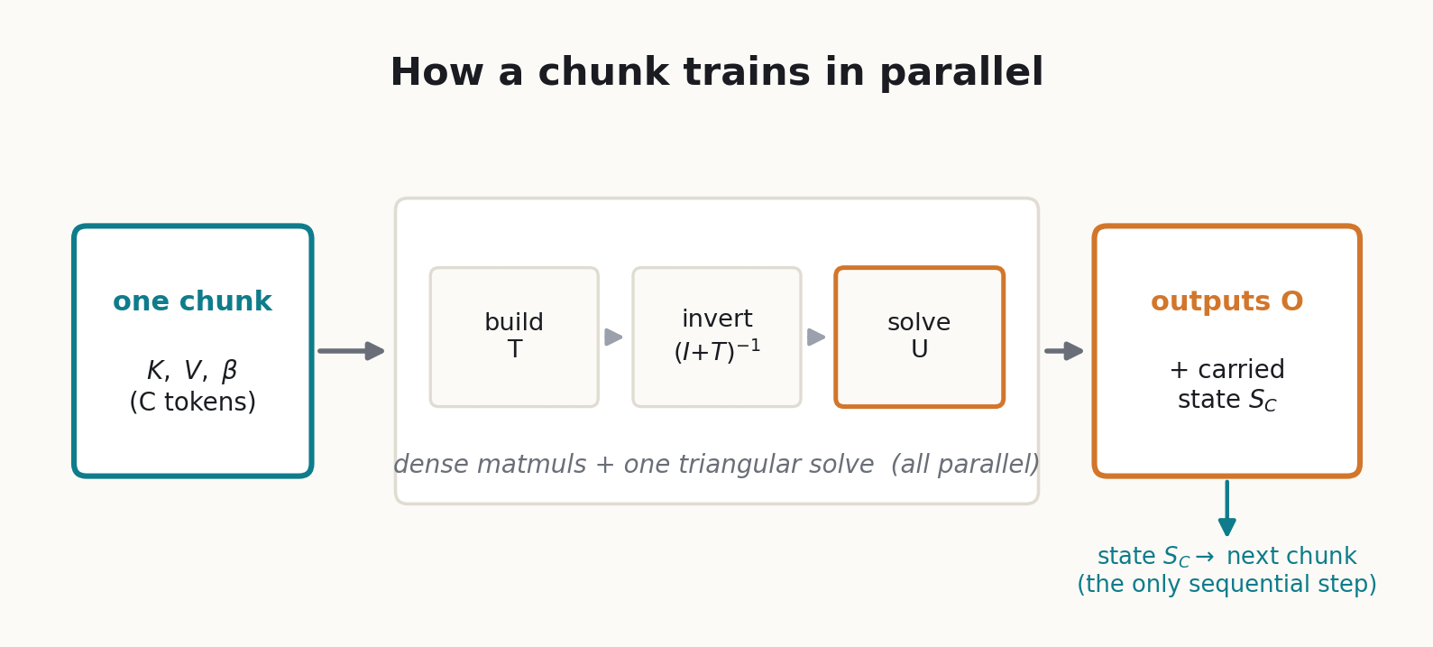
The delta rule looks sequential but trains in parallel as one small triangular solve per chunk.
Decay, then per-channel decay (KDA), then decoupled erase/write gates (GDN-2) are three refinements that keep that solve intact.
Which memory we mean
“Memory” means three different things in a language model. This post is about one of them.
The weights. The query/key/value projection matrices and the gates, learned during training and fixed afterward. Long-term knowledge, changed only by more training. Not this.
The KV cache (softmax). The full list of past keys and values, so any query can look back exactly. Lossless, grows with context, reset each sequence. Linear attention removes this.
The recurrent state (linear attention). One fixed-size matrix summarizing every token so far. Lossy, fixed size, reset each sequence. This is the memory we mean.
So this is in-context memory: holding the current input within a single forward pass, so token 5,000 can use what token 3 said. New prompt, empty state, nothing saved. It is not retrieval/RAG, not continual learning, not “remembering you across sessions”; it is the job plain attention does with its KV cache, just compressed into a fixed matrix instead of a growing list.
Where the state comes from
Each token has a representation, and three fixed learned matrices turn it into a query, a key, and a value:
The key is a token’s address, what it is about; the value is the content stored there; the query is what the current token is asking for, matched against the keys to decide what to pull out. A token writes itself in as a key–value pair and later reads with a query. The vectors depend on the input, but the three projection matrices are fixed weights, shared across every position and sequence.
Ordinary attention computes each output as a softmax-weighted sum over the past:
The exponential is what forces the cache. The score exp(query · key) does not split into a part that depends only on the query times a part that depends only on the key, so the weight on each value is tied to that specific key, and the normalizer sums over every past key. There is no running summary you can keep instead: you have to store every key–value pair and revisit them for each new query. That is the KV cache: memory grows linearly with sequence length, and producing all outputs scales quadratically with it.
Linear attention drops the softmax and uses a score that factorizes, in the simplest case just the dot product of query and key. Once it factorizes, the sum rearranges:
All of history collapses into one matrix of fixed size (key-dimension by value-dimension), and the query reads it in a single multiply. Memory no longer grows with context and the per-token cost is constant. This fixed state is the object the rest of this post is about; it exists precisely because the softmax is gone.
That fixed size is the appeal and the problem at once. Packing an unbounded history into one matrix is cheap, but it means many facts share the same finite space. The next section shows what that does to a read.
Why a fixed-size memory interferes
We have the fixed-size state. Before writing into it, look at what reading it gives you. Reading is applying a query to the memory:
Each stored value is weighted by how aligned its key is with the query, the dot product of the two. That is content-addressed recall: values whose keys match what you asked for, weighted by the match.
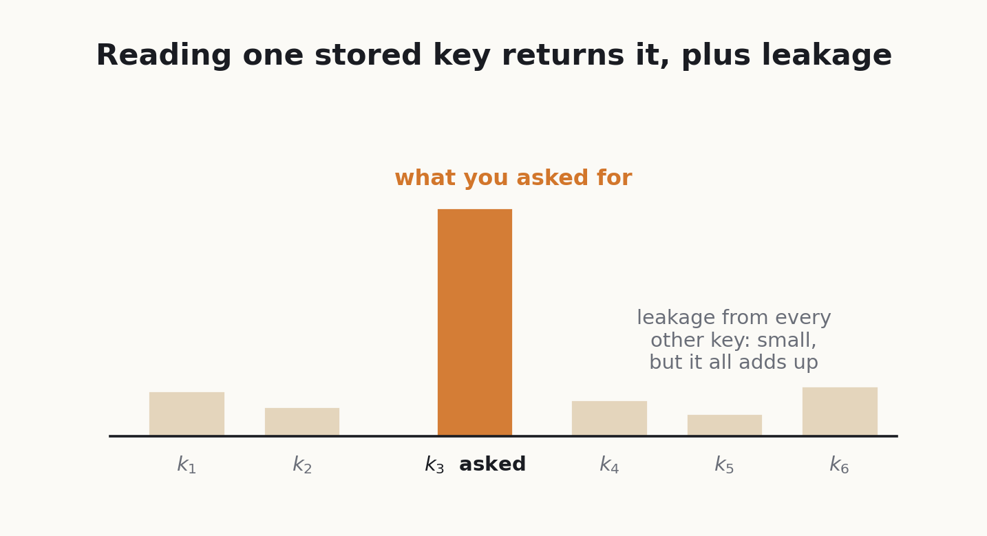
To expose the problem, take the cleanest possible query, one that exactly equals a key you already stored. This is the case that should return its value perfectly, so any mess is the memory’s fault, not a mismatched query. Splitting off that term:
If the stored keys were orthonormal, every cross term would be zero and the read would be clean. They are not. Each nonzero overlap leaks a fraction of some other value into the answer. And here is the structural reason they cannot all be orthogonal: the state is a single matrix, so the key space has only as many dimensions as the key vector is wide, and a space of that dimension holds at most that many mutually orthogonal directions. Store more associations than that and some keys must share directions; even below the limit, random unit keys have small but nonzero overlaps that add up.
As the context carries more associations, the term you want stays about the same size while the leakage is a sum over everything else, so it grows. Signal-to-noise falls with context length: a long document forces many distinct facts to share one fixed box and they smear together. That is why this whole family struggles on long, many-needle retrieval, and why the improvements below all aim at that pressure point.
Why softmax doesn’t have this problem
The leakage is not caused by folding the sum into the state matrix. The summed form and the matrix form are the same number; folding only fixes the size and the cost, not the value. The leakage is already there in the raw dot-product score.
Softmax runs those same dot products through an exponential and normalizes. The exponential sharpens them: the matching key saturates near one and the mismatched keys are crushed toward zero, so the wrong values effectively drop out of the read even when the keys overlap. Same overlaps, clean answer.
But that is exactly the property that cannot be summarized. The exponential of a dot product does not split into a query part times a key part, so there is nothing to precompute: you are forced to keep every key and recompute the exponential against each one, which is the growing cache. So it is an either/or: a sharp score reads cleanly but cannot be folded into a fixed state, while a foldable score gives the fixed state but leaks. Interference is not the cost of compressing; it is the cost of using a score weak enough to be compressible.
Updating a value when a key comes back
As the model reads a sequence, a later token sometimes produces a key close to one an earlier token already wrote, but carrying a different value. The state already holds a binding in that direction, and the new value should take its place. This is the update case, and it is the one ordinary outer-product memory gets wrong.
For example, a passage sets x = 5 and later sets x = 7. Both tokens produce nearly the same key (the direction standing for “the value of x”), but with different values. When a later token reads x, the answer should be 7. Plain addition cannot give that: it never removed the old binding, so the slot holds 5 and 7 at once and the read returns a blend. The same shape shows up whenever a key recurs with a new value: an entity whose state changes (”Alice is in Paris… now Tokyo”), a correction (”blue… actually green”), a form field revised.
Two clarifications, since “update” can mislead. The prompt itself is fixed; the forward pass only reads it left to right, and “update” means a later position’s binding should win over an earlier one. “x = 5” stays in the text; it just should not win the read. And keys are not matched by name: two tokens are “the same key” when their key vectors point in roughly the same direction, so their writes land on the same spot in the state. A repeated mention produces a nearby key, the later write hits that slot, and the read afterward should reflect the new value.
So every write is one of two cases. Add: the key points somewhere new, a fresh fact, which is most tokens; plain accumulation is fine, and that is what vanilla linear attention does. Overwrite: the key lands on a direction already in the state, and the slot has to be updated to the new value, not stacked on top of the old one.
Why not just replace the whole matrix?
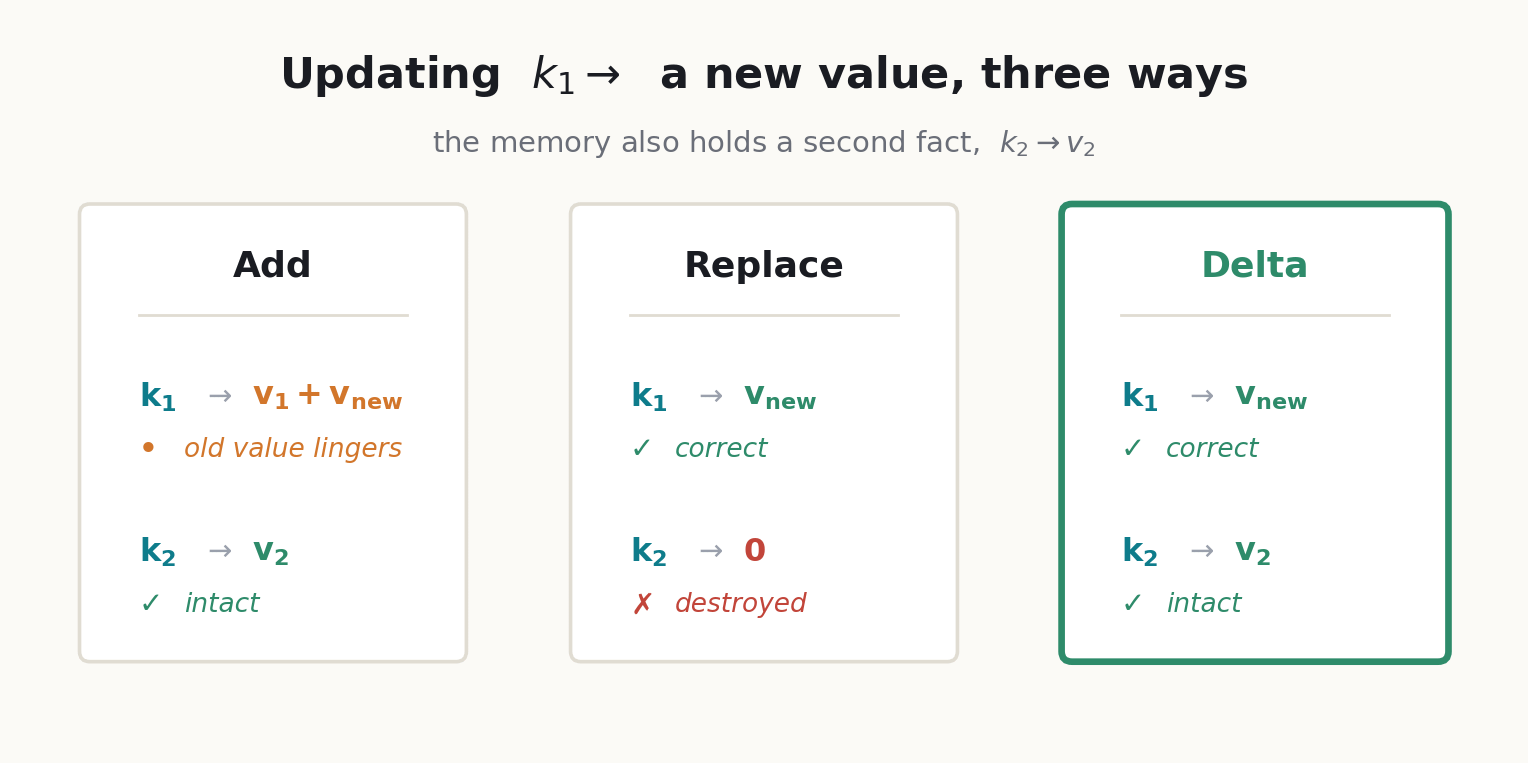
Because the state is shared by every association at once. Three ways to write an update to one key, into a memory that also holds a second fact:
Replace the whole matrix with the new key–value outer product: fixes the target key perfectly and deletes everyone else. Read the second key afterward and you get near zero. You wanted to change one slot and you erased the notebook.
Add the new outer product: keeps the second fact, but leaves the old binding in place, so reading the target key returns old-plus-new, the stale value smeared into the fresh one.
Delta: read what the key currently points to, subtract just that, then write the new value. Only the target slot changes; the other fact is untouched.
Add keeps the other fact but smears the target. Replace fixes the target but wipes the other fact. Only the third (read, subtract, write) gets both right. That third option is the delta rule.
The delta rule
The update that does this is the delta rule (Widrow & Hoff, 1960), used for linear attention in DeltaNet (Yang et al., 2024). It writes the new value relative to what is already stored, not absolutely. First read what the memory currently returns for the key:
This is whatever sits in that key’s direction right now. We never have to know in advance whether the key was used before; we just read it back. Then move the slot from that old value toward the target, by a fraction β (the write strength):
The bracket is the gap between the new value and the old one, and adding it back pushes the value stored at that key toward the target. One update covers both cases with no branching: if the key points somewhere new, the read is about zero, the gap is just the new value, and it reduces to a plain add; if the key lands on a direction that already holds a value, the read returns that old value, and the update subtracts it and writes the new value in its place. The memory tells the rule which case it is in.
Multiplying the correction out shows what it does to the whole state:
The second term writes the new value along the key. The first term removes a β fraction of whatever the state held along that key, and only along that key: the projection onto the key direction leaves everything orthogonal to it untouched. That is exactly why, in the previous widget, replacing the whole matrix wiped the bystander but the delta update did not; it only edits that one key’s line of the state.
Why β is not just 1
A write strength of 1 is a hard overwrite: erase the old binding completely, write the new value. So why not use it everywhere? β is produced per token by the model, and two things argue against pinning it to 1. Real keys are not exactly orthogonal, so erasing hard along one key also disturbs neighbors that partly share its direction, and a smaller β makes a gentler edit with less collateral damage. And not every write should fully replace: sometimes the right move is to nudge a value, accumulate evidence, or write weakly under uncertainty. So β between 0 and 1 is a dial: 1 overwrites, 0 leaves the slot alone, in between is a partial move. (In the online-learning view it is a per-step learning rate, and a rate of 1 everywhere is rarely what you want.)
One caveat the next widget makes concrete: the clean overwrite is exact only when the key is orthogonal to the others. When keys overlap, editing along one drags on whatever shares its direction, the same interference from before, now showing up in the write.
Training it in parallel
Training needs every output over the whole sequence at once, then a gradient. Plain linear attention gives them cheaply because the state is a running sum, so the outputs collapse into two matrix multiplies (with a causal mask zeroing the future):
Why this is fast: it is all dense matmuls, and a GPU runs a matmul as thousands of multiply-adds in parallel on its tensor cores, every output position at the same time. Nothing waits for anything else.
The delta rule breaks this. Its erase factor (the one from the operator form above) makes each state genuinely depend on the previous one, so you cannot write the answer as one sum of independent terms. Done literally you process tokens one at a time, each a tiny rank-one update that uses a sliver of the GPU while the rest sits idle.
DeltaNet’s contribution (Yang et al., 2024) was to recover the matmul form by working in chunks. A chunk is a contiguous block of C tokens; a length-L sequence is split into L/C of them. The expensive work happens inside a chunk, all as matmuls, and only a small summary state is passed from one chunk to the next.
The trick: solve for the values that were actually written
Every step adds a rank-one term whose left factor is a key, so the state is always the start state plus one such term per token:
The written value here is not the raw value, but the correction from the delta rule (target minus old value, scaled by β). The keys are known; these written values are the unknowns. The point is that if we can get all of them in a chunk at once, with a single matrix solve instead of a token-by-token walk, the whole chunk becomes parallel matmuls. So we solve for them jointly.
The written value at each step depends on the current read, and that read expands into known keys and earlier written values:
In words: reading a key against the state-so-far is the start-state read, plus every earlier written value weighted by how much its key overlaps the current one. Substituting gives a relation among the written values alone:
Each written value depends only on earlier ones, which makes this a triangular system. Stack the written values into a matrix, collect the pairwise key overlaps into a matrix T, and the whole set of equations becomes a single solve:
Because the matrix being inverted is unit lower-triangular, the inverse is one forward substitution on a small C-by-C matrix. Everything else is dense matmuls: build the overlap matrix from pairwise key dot products, then form the carried state and the outputs:
The sequential token loop is gone, replaced by matmuls plus one small triangular solve. Writing a product of rank-one factors as a single low-rank update this way is a classical move from numerical linear algebra, the WY representation (Bischof & Van Loan, 1985) and its UT-transform variant (Joffrain et al., 2006); DeltaNet borrows it to collapse the chunk into matrix operations.
Why the chunk size is small
The chunk size sets how often the state is handed off: there are L/C chunks, so that many sequential state updates. The two extremes make this concrete. A chunk of one token is the original fully sequential recurrence. A single chunk covering the whole sequence is one handoff, done in one parallel block. (This is the opposite of what it might sound like: a bigger chunk means fewer, larger steps, not more.)
So why not use one giant chunk and be fully parallel? Because the chunk builds and solves a C-by-C matrix, so its cost and memory grow quadratically in the chunk size. At the full length you are back to the quadratic cost of full attention, and the matrix no longer fits in the fast on-chip memory the matmul engine reads from. Too small, and you pay too many sequential steps and underfill each matmul. The kernels use 64.
Adding decay: Gated DeltaNet
Everything up to here is DeltaNet: a fixed-size associative memory, edited by the delta rule, trained in parallel. The last three sections are refinements, each adding expressive power with a small change that leaves the chunk algorithm intact.
The delta rule overwrites one slot at a time but cannot let old context fade on its own. Gated DeltaNet (Yang, Kautz & Hatamizadeh, 2025, arXiv:2412.06464) multiplies the state by a scalar decay before each edit:
Tracking the cumulative product of the decays, an earlier write contributes to a later read scaled by how much decay has accumulated in between. In the chunk algorithm this is just a per-row reweighting of the same matrices plus an extra factor in the causal mask; the triangular solve is unchanged. Decay is close to free to add. What it cannot do is forget different features at different rates, since it is one number.
Decay per channel: KDA
KDA, the linear-attention layer in Kimi Linear (Kimi Team, 2025, arXiv:2510.26692), replaces that single decay with a per-channel decay vector, a different forget rate for every key channel:
Now every channel is scaled differently at every step, which looks like it should break the chunk form. It does not, because of a change of variables: factor the cumulative per-channel decay out of the state, and it cancels from the recurrence, leaving a plain delta product in reweighted key and erase factors:
After this substitution the chunk equations have the same shape as before; only the entries carry the decay factors. KDA buys richer forgetting at no structural cost.
The per-channel rates are not hand-set hyperparameters; they are learned and data-dependent, produced from each token by a small projection (the Gated DeltaNet parameterization, a softplus of a learned linear map passed through an exponential). A per-head term and a per-channel bias set each channel’s baseline forget rate, and the per-token projection pushes that rate up or down, so the model learns both the typical decay profile and how to modulate it on the fly. The active edit, though, is still a single write-strength scalar, which scales both the erase and the write at once.
Splitting the edit: Gated DeltaNet-2
Erasing acts on the key side: which coordinates of the old read to remove. Writing acts on the value side: which coordinates of the new value to keep. These are different axes of the state, so GDN-2 (Hatamizadeh, Choi & Kautz, 2026, arXiv:2605.22791) gives each its own channel-wise gate, an erase gate on the key and a write gate on the value:
Compared with KDA, the write direction is unchanged (the left factor is still the key), but the read it subtracts is now channel-selected by the erase gate, and the value it writes is channel-selected by the write gate.
Forward: same machine
Run the same change of variables, now folding the erase gate into the reweighted factor, and the recurrence is again a plain (now asymmetric) delta product. The chunk pipeline keeps the same shape: the same overlap matrix, the same triangular inverse, the same state and output equations. The only difference is what fills them: the erase gate enters the key-side rows, the write gate the value-side rows, and the overlap matrix is now built from an asymmetric pair rather than a symmetric one.
Backward: one real difference
Training propagates a loss gradient back through the chunk. Write the solve as the triangular inverse applied to the written values. Backprop needs the gradient with respect to that inverse, which accumulates as a product of the incoming gradient with the written values:
The whole question is whether the gate can be pulled out of that inner product. In KDA the written value is a scalar times the value, so it slides straight out, and you can compute the gate-free products once as a matmul and scale afterward:
In GDN-2 the written value is a per-channel product, so the gate sits inside the sum over channels and there is nothing to pull out:
No single number multiplies the whole inner product; the gate reweights each channel before it is summed, so no row or column scaling recovers it from the gate-free version. The erase side has the same issue. The gate therefore has to be folded into the matmul itself, not applied as a scaling after. The forward pass is essentially KDA’s; the backward kernel is the part that must be rewritten to carry both gates inside its accumulation, and that gate-aware backward is the real implementation cost of the split.
Setting both gates to the same scalar recovers KDA exactly; tying the decay to a scalar as well gives Gated DeltaNet; dropping the decay gives the delta rule. Each model is the next with some gate held to a scalar.
Where this nets out
Step back and it is all one idea, taken in stages. Linear attention compresses an unbounded history into a fixed matrix, fast but lossy. The delta rule edits that matrix surgically instead of piling onto it. The chunked triangular solve makes the edit trainable at scale. Decay, per-channel decay, and decoupled erase/write gates each give the edit finer control over what to keep and what to remove, without giving up the fixed-size state or the parallel training. None of them recover the softmax cache's perfect recall; they make the compression smarter.
That is also where the measured gains land. In the Gated DeltaNet-2 paper the improvement over KDA is modest on language modeling but clear on long-context, multi-key retrieval, the regime where many associations are forced to share one fixed state and interference is worst. The ablation is honest about the split: a channel-wise erase gate with a scalar write recovers most of the gain, so the erase side is doing more work than the write side.
This is also why pure linear attention rarely replaces softmax outright. Exact recall is often worth the cost of the growing cache, so most production models stay softmax, and these layers show up where memory and throughput dominate: long context, high-throughput serving, constrained hardware. The common deployment is hybrid: interleave a few full or sliding-window attention layers for exact recall with many cheap linear layers. Recent open-weight models make this concrete. Qwen3-Next and Kimi Linear both stack three linear blocks (a Gated DeltaNet variant) per full-attention block, a 3:1 ratio, and MiniMax-01 mixes lightning (linear) and softmax attention in a similar pattern.
Sources:
DeltaNet chunkwise algorithm (Yang, Wang, Zhang, Shen, Kim, NeurIPS 2024)
Gated DeltaNet (Yang, Kautz, Hatamizadeh, ICLR 2025, arXiv:2412.06464);
KDA / Kimi Linear (Kimi Team, 2025, arXiv:2510.26692);
Gated DeltaNet-2 (Hatamizadeh, Choi, Kautz, 2026, arXiv:2605.22791).